Kamagra repose sur le sildénafil comme principe actif, avec un mode d’action identique à celui du Viagra. La forme galénique en gel oral permet une absorption plus rapide et une concentration plasmatique maximale plus précoce que les comprimés. Le mécanisme implique l’inhibition compétitive de la PDE5, entraînant une relaxation musculaire lisse locale et une vasodilatation ciblée. La demi-vie courte, environ 4 heures, limite la durée d’action. L’élimination se fait après métabolisme hépatique, impliquant majoritairement le CYP3A4. L’incidence d’effets indésirables comprend céphalées, rougeurs et congestion nasale, de façon transitoire. Dans les comparatifs pharmacologiques, acheter kamagra sans ordonnance est associé aux présentations galéniques alternatives disponibles.
Users.physik.fu-berlin.de
Three-loop ground-state energy of O„N…-symmetric Ginzburg-Landau theory above Tc in 4- dimensions with minimal subtraction Institut fu¨r Theoretische Physik, Freie Universita¨t Berlin, Arnimallee 14, D-14195 Berlin, GermanyPhysique Nucle´aire The´orique, B5, Universite´ de Lie`ge Sart-Tilman, 4000 Lie`ge, Belgiumand Institut fu¨r Theoretische Physik, Freie Universita¨t Berlin, Arnimallee 14, D-14195 Berlin, Germany
͑Received 1 October 2001; published 19 April 2002͒
As a step towards deriving universal amplitude ratios of the superconductive phase transition we calculate
the vacuum energy density in the symmetric phase of O(N)-symmetric scalar QED in Dϭ4Ϫ dimensions inan expansion using the minimal subtraction scheme commonly denoted by MS. From the diverging parts ofthe diagrams, we obtain the renormalization constant of the vacuum Zv which also contains information on thecritical exponent ␣ of the specific heat. As a side result, we use an earlier two-loop calculation of the effectivepotential ͓H. Kleinert and B. Van den Bossche, cond-mat/0104102͔ to determine the renormalization constantof the scalar field Z up to two loops.
PACS number͑s͒: 74.20.De, 64.70.Ϫp, 05.70.Jk
I. INTRODUCTION
vation was made by Nogueira,14 that an anomalous momen-tum instability below Tc may be responsible for the unusual
One of the most intriguing problems in the physics of
resistance of the superconductive transition to theory. Hope
critical phenomena is a theoretical understanding of the su-
for a better understanding has also been raised by a recent
perconductive phase transition within the renormalization-
renormalization-group study in dϭ3 dimensions performedbelow T
group approach. A discussion was given in 1974 by Halperin,
c where a fixed point has been found at the one-loop
Lubensky, and Ma2 on the basis of the Ginzburg-Landau or
Once an infrared-stable fixed point is located, it will de-
Abelian Higgs model, in 4Ϫ⑀ dimensions, generalizing a
termine critical exponents and amplitude ratios. The former
can be extracted from the perturbative expansions of the
Weinberg.3 In a one-loop approximation, they did not find an
renormalization constants corresponding to coupling, mass,
infrared-stable fixed point, and in spite of much effort it is
and wave-function renormalization. The latter also requires
still unclear whether a higher-loop renormalization-group
the calculation of finite parts of certain quantities. For in-
analysis would be capable of explaining the existence of a
stance, the amplitude ratios for the specific heat can be ob-
critical point in 4Ϫ dimensions. Experimentally, this exis-
tained by computing both the divergent and finite parts of the
tence has been confirmed only recently with the advent of
vacuum energy in the symmetric and in the symmetry-
c superconductors. In conventional superconductors,
Our work will provide analytic results for the divergent as
the Ginzburg criterion,4 or the more relevant criterion for the
well as finite parts of the vacuum energy up to three loops in
size of phase fluctuations,5 predicted a too small temperature
the symmetric case. While the divergent part is the same in
interval for the critical regime to observe anything beyond
the symmetry-broken case, the determination of the finite
mean-field behavior. Evidence had so far come only from
part in that case is left for future work.
Monte Carlo simulations6 and an analogy with smectic-
We work with the so-called modified minimal subtraction
nematic transitions in liquid crystal.7 Only by artificially al-
scheme, denoted by MS.16 The singularities are collected in
lowing for an unphysically large number of replica n of the
the dimensionless renormalization constant Zv . In the course
complex field , larger than 365, has it been possible to
of the calculations, we also recover information about the
stabilize the renormalization flow in 4Ϫ dimensions. His-
other renormalization constants of the theory. This may be
torically, a dual disorder formulation of the Ginzburg-Landau
viewed as a cross check of our work.
model brought in 1982 theoretical proof for the existence of
Since the theory has so far only a fixed point for large n
a tricritical point at a Ginzburg parameter ͱ2Ϸ0.77, a ma-
Ͼ365, we shall keep an arbitrary number of replica in the
terial parameter characterizing the ratio between magnetic
theory, the physical case being nϭ1. The n complex fields
and coherence length scales.8,9 This prediction was recently
are coupled minimally to an Abelian gauge field which de-
confirmed by extensive Monte Carlo simulations.10
scribes magnetism. The Nϭ2n real and imaginary parts of
The confusing situation in the Ginzburg-Landau model
the fields are assumed to have an O(N)-symmetric quartic
certainly requires further investigation in higher loop ap-
proximations. So far, two loop renormalization-group calcu-lations in 4Ϫ dimensions have not yet produced satisfac-
II. MODEL
tory results.11,12 Analyses in dϭ3 dimensions a` la Parisi
The Lagrangian density to be studied contains nϭN/2
have also left many open questions.13 An interesting obser-
complex scalar fields B coupled to the magnetic vector po-
0163-1829/2002/65͑17͒/174512͑7͒/$20.00
65 174512-1
PHYSICAL REVIEW B 65 174512
tential AB and reads, with a covariant gauge fixing,
normalization factor as the field itself, going over into
ͱZD. An arbitrary mass scale in Eq. ͑3͒ serves to
define dimensionless coupling constants g and e.
The above multiplicative renormalizations are not suffi-
cient to extract all finite information from the theory. The
vacuum energy requires a special treatment, as emphasized
in a previous work of one of the authors ͑B.K.͒.21 Dimen-sionality requires the effective potential to have mass dimen-
where DBϭץϪieBAB denotes the covariant derivative,
sion D. To have a finite vacuum energy we must add to the
FBϭץABϪץAB is the field strength, and ␣ a gauge
parameter. The bare character is indicated by the subscript‘‘B.’’ In principle, there are also ghost fields which, however,
decouple in the symmetric phase and remain massless. Work-
ing in dimensional regularization they do not contribute to
The different renormalization constants may be expanded in
powers of the fluctuation size ប as follows:
The coefficient 1/4 in front of the coupling constant g
conventional. The Feynman diagrams associated with the
vacuum energy of the Lagrangian ͑1͒ have been generated
where the subscript j stands for fields and coupling constants
iteratively in Ref. 17. At some places it will be useful to
,A,m,g,e. In minimal subtraction, each expansion coeffi-
compare our results with those of an earlier work,1 where we
have derived the two-loop effective potential above and be-low Tc . For such comparisons, a replacement g B
ϭ ͚ glϪke2k͑c Ϫlϩc 1Ϫlϩ•••ϩc Ϫ1͒,
A full extension of the work in Ref. 1 is highly nontrivial
since the effective potential requires the calculation of Feyn-man diagrams with three different masses. For this reason we
except for Z(l) , where the systematics is
shall restrict ourselves in this paper to the symmetric phaseTϾTc , where the field expectations vanish and the system
contains only two masses, which greatly simplifies the prob-
ϭ ͚ glϩ1Ϫke2k͑c Ϫlϩc 1Ϫlϩ•••ϩc Ϫ1͒,
lem, in particular since one of the masses, the photon mass,
is zero. As a consequence, most diagrams can be reduced toscalar integrals which can be computed exactly. The only
exception is the watermelon—or basketball—diagram whose
expansion is, however, known to sufficiently high order in
glϪ1Ϫke2k͑cv
As in Ref. 1 we shall use throughout Landau gauge ␣
→0, which enforces a transverse photon field. This has theadvantage of being infrared stable.19,20
Initially, one finds also pole terms of the form 1/2ϫln,1/ϫln, and 1/ϫln2, where ln is short for ln(m2/
III. RENORMALIZATION
being related to the mass scale via the Euler-Mascheroniconstant ␥
The renormalization constants of the model are defined by
¯ 2ϭ42exp(Ϫ␥E). These, however, turn
out to cancel each other, which provides us with a nice con-sistency check of the renormalization procedure.22
IV. FEYNMAN RULES AND VACUUM DIAGRAMS
The elements of the Feynman diagrams associated with
where, in the last equation, we have taken into account the
Z , which is a consequence of the Ward iden-
tity. Heuristically, this equality comes from the requirementthat the covariant derivative DBB should not only be in-
variant with respect to gauge transformations but also with
ϭ Ϫpp /p2 ,
respect to renormalization. Thus it must acquire the same
THREE-LOOP GROUND-STATE ENERGY OF O(N)- . . .
PHYSICAL REVIEW B 65 174512
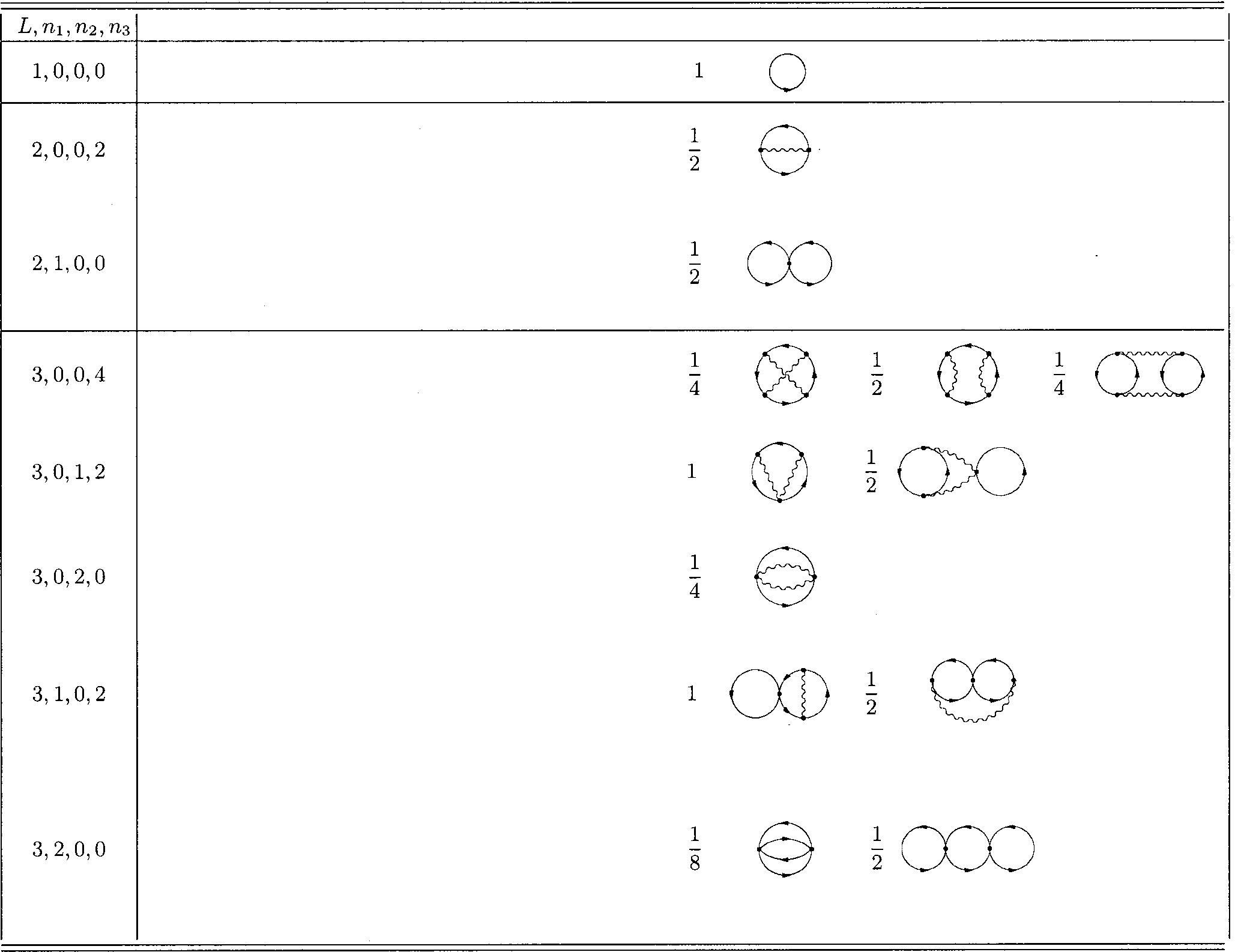
TABLE I. Relevant one-particle irreducible vacuum diagrams W(L,n1 ,n2 ,n3) and their weights through three-loop order of the O(N)
Ginzburg-Landau model, where L denotes the loop order and n1 ,n2 ,n3 count the number of g,e2, and e vertices, respectively.
In Ref. 17, the vacuum diagrams of the theory have been
generated recursively up to four loops. Table I shows alldiagrams needed for the three-loop vacuum energy above
c , omitting those which contain massless separable loop
integrals which vanish by Veltman’s rule ͑2͒. g2͑Nϩ5͒Ϫ3ge2ϩ6e4ͬ
V. RENORMALIZATION CONSTANTS Z„3… v AND Z
The determination of the two-loop effective potential be-
allows us to extract the following one- and two-loop
g2͑Nϩ2͒Ϫ2ge2͑Nϩ2͒Ϫe4͑5Nϩ1͒ͬ,
contributions to the renormalization constants. Note that afactor (4)Ϫ2l has been taken out in the definition ͑5͒,
PHYSICAL REVIEW B 65 174512
ͩe␥EͪϪ3/2ͫ 208 188 179ϩ26͑2͒
g3͑Nϩ8͒2Ϫ3g2e2͑Nϩ8͒
12ge4͑Nϩ8͒ϩ8e6͑Nϩ18͒ͬ
g3͑5Nϩ22͒Ϫ2g2e2͑Nϩ5͒
2ge4͑5Nϩ13͒ϩ e6͑7Nϩ90͒ͬ,
3e2ϩ g͑Nϩ2͒ͬϩ2e2
A. Results for the Feynman integrals
In this section, we give the value of the diagrams listed in
Table I. Although the exact value of part of the three-loop
diagrams is known, we only give the expansion throughorder 0, for the sake of brevity. The notation is as follows:
Iln is the integral for the case Nϭ2, omitting the weights of
ϫͫϪ Ϫ Ϫ Ϫ22Ϫ6͑2͒ϩ3͑3͒ͬ,
Table I and setting coupling constants and scalar mass equal
to unity. The first index l is the loop order while the second
index n counts through the diagrams within each loop orderas listed in Table I.
ͩe␥EͪϪ3/2ͫ8 28 5ϩ3͑2͒
ͩe␥EͪϪ3/2ͫ24 40 50ϩ9͑2͒
ͩe␥EͪϪ3/2ͫ96 242 6
where Li4 in Eq. ͑25͒ denotes the polylogarithm of order 4:
THREE-LOOP GROUND-STATE ENERGY OF O(N)- . . .
PHYSICAL REVIEW B 65 174512 B. Divergent terms through three loops
to 1/2ϫln gives Z(1,1) as a function of Z(1,1) and Z(1,1) .
Inserting this into the expression for Z
vac the vacuum energy density in the sym-
metric phase, we find up to three loops the expansion
ϭe4͑6Ϫ5N͒ϩ6e2Zm2
Ϫͫ3 g2͑Nϩ2͒ϩ g͑Nϩ2͒Z(1,1)ϪZ(2,2)ͬ.
Taking into account all these relations, the 1/ ⑀n pole terms
are found to be removed with Z(3,1)
Using the known results for Z(1,1) and Z(1,1) , we recover
the result ͑15͒ derived before in Ref. 1. Using the known
coinciding with previous results derived from a renormaliza-
tion of the two-point functions in Refs. 11 and 24.
Finally, inserting Z(1,1) into Z(3,1) and Z(3,2) , we have
N͓43Nϩ294Ϫ384͑3͔͒e4
A few remarks are useful on the calculation of the pole terms
of the diagrams. Taking into account the expansion of therenormalization constants in the form ͑5͒, each Feynman in-
tegral is expanded up to order ប3. The expansion coefficients
are determined to cancel the 1/n terms arising from the
Feynman integrals. In particular we have:
To order ប, the cancellation of the 1/ pole leads directly
N͑Nϩ2͒͑Nϩ4͒g2
to the known one-loop result ͑18͒ as in Ref. 1; to order ប2,
there are pole terms of the form 1/2, 1/, and 1/ϫln. The1/ϫln terms cancel if
For e2ϭ0 we recover the three-loop result of the pure 4
which is fulfilled by the one-loop expressions ͑14͒ and ͑16͒
for Z(1) and Z(1) , respectively. After this, the cancellation of
the ordinary poles lets us recover the result ͑21͒ obtained
VI. RENORMALIZATION-GROUP FUNCTION OF THE VACUUM ␥
Finally, we need to cancel the poles at the ប3 level. Be-
v
sides poles without logs, there are poles of the types 1/
The critical behavior of the renormalization constant Zv is
ϫln, 1/2ϫln, and 1/ϫln2, which have to vanish. To sim-
characterized by the finite renormalization-group function ␥v
plify the discussion, we introduce the notation Z(i, j) where
the first superscript i indicates the loop order, and the secondsuperscript j gives the order of the pole, i.e., Z(i)
Z(i, j)/ j.
When removing the pole proportional to 1/ϫln2 we ob-
Using standard methods,25 ␥v can be extracted from the
Similarly, the removal of 1/ϫln gives Z(2,1)
simple pole terms of Zv , whose residue will be denoted by
Z(1,1) and Z(2,1) . Finally, the removal of the pole proportional
PHYSICAL REVIEW B 65 174512
The results of the last section for the Z(l,1)
ϩ24͑3͒ͬe4ͮͫ ប ϩO͑ប4͒. VII. VACUUM ENERGY DENSITY
In the previous section, we have focused on the removal
E ϭͩ Nϩ2 gϪ3e2ͪln2ͩ m2 ϪͩNϩ2 gϪ14e2ͪ
of divergences, thus fixing the renormalization constants.
Since the three-loop integrals I3a—I3j are known to zerothorder in 0, we can also determine the finite vacuum energy
density of the symmetric phase of the Ginzburg-Landau
model. Up to a negative sign, it is given by the sum of thevacuum diagrams. Having in mind the application of ourresult to phase transitions in three dimensions, we give here
its expansion. We must calculate the one-loop diagram up
to the order 2 and the two-loop diagrams up to the order .
The general form of the L-loop result has an expansion
4 lϭ1 ͑4͒2 kϭ0
where we have assumed that e2 and g are of order , whichis correct at the fixed point relevant for the neighborhood of
the phase transition. The expansion coefficients are
E ϭͫ͑Nϩ2͒͑Nϩ4͒
e4ͬln2ͩ m2 ϩͫ͑Nϩ2͒͑2Nϩ39͒ g2Ϫ
g2ϩ6͑Nϩ2͒ge2ϩͫ1351N ϩ
Ϫͩ56N ϩ208 ͑3͒ϩ176͑4͒ϩ64͑2͒ln22Ϫ ln42Ϫ256Li
VIII. CONCLUSION
plitude ratios of the specific heat at the phase transition of themodel.
With the help of dimensional regularization and the modi-
To arrive at the final goal of deriving universal amplitude
fied minimal subtraction scheme MS we have computed the
ratios for the specific heat above and below the phase tran-
vacuum energy density in an expansion up to three loops
sition, we must perform a similar calculation also in the or-
for the symmetric phase of the Ginzburg-Landau model. Fur-
dered phase below Tc . Such a calculation will be compli-
ther, we have determined the renormalization-group function
of the vacuum ␥v , which is the same above and below Tc .
appearance of more mass scales and infrared divergences for
Both quantities will be needed for the calculation of the am-
NϾ2. Fortunately, the amplitude ratio of the specific heat
THREE-LOOP GROUND-STATE ENERGY OF O(N)- . . .
PHYSICAL REVIEW B 65 174512
does not require knowledge of the full effective potential, but
ACKNOWLEDGMENTS
only its value at the minimum, whose evaluation is simplerand will be given in future work.
Certainly it is hoped that a higher loop effective potential
We thank Dr. D. J. Broadhurst, Dr. J.-M. Chung, and Dr.
describing the phase transition will give us specific informa-
B. K. Chung for helpful communications. The work of B.
tion on the nature of the superconductive phase transition, in
VdB. was supported by the Alexander von Humboldt foun-
particular on the value of the Ginzburg parameter at which
dation and the Institut Interuniversitaire des Sciences Nucle´-
under the supervision of one of the present authors ͑H.K.͒.
12 R. Folk and Y. Holovatch, J. Phys. A 29, 3409 ͑1996͒.
2 B.I. Halperin, T.C. Lubensky and S.-K. Ma, Phys. Rev. Lett. 32,
13 C. de Calan and F.S. Nogueira, Phys. Rev. B 60, 4255 ͑1999͒.
292 ͑1974͒; J.-H. Chen, T.C. Lubensky and D.R. Nelson, Phys.
14 F.S. Nogueira, Phys. Rev. B 62, 14559 ͑2000͒.
Rev. B 17, 4274 ͑1978͒.
15 H. Kleinert and F.S. Nogueira, cond-mat/0104573 ͑unpublished͒.
3 S. Coleman and E. Weinberg, Phys. Rev. D 7, 1888 ͑1973͒; For a
16 For the definition of various subtraction schemes, see H. Kleinert
comparison of the two theories see H. Kleinert, Phys. Lett.
and V. Schulte-Frohlinde, in Critical Properties of 4-Theories128B, 69 ͑1983͒͑http://www.physik.fu-berlin.de/ϳkleinert/106͒.
͑World Scientific, Singapore, 2001͒, Chap. 13, pp. 1–487 ͑http://
4 V.L. Ginzburg, Fiz. Tverd. Tela ͑Leningrad͒ 2, 2031 ͑1960͒ ͓Sov.
www.physik.fu-berlin.de/ϳkleinert/b8͒.
Phys. Solid State 2, 1824 ͑1961͔͒; See also the detailed discus-
17 H. Kleinert, A. Pelster, and B. Van den Bossche, hep-th/0107017
sion in Chap. 13 of the textbook L.D. Landau and E.M. Lifshitz,
Statistical Physics, 3rd ed. ͑Pergamon Press, London, 1968͒ and
18 D.J. Broadhurst, Z. Phys. C 54, 599 ͑1992͒; D.J. Broadhurst, Eur.
by C.J. Lobb, Phys. Rev. B 36, 3930 ͑1987͒.
Phys. J. C 8, 311 ͑1999͒; J.-M. Chung and B.K. Chung, J. Ko-
5 H. Kleinert, Phys. Rev. Lett. 84, 286 ͑2000͒.
rean Phys. Soc. 38, 60 ͑2001͒.
6 J. Bartholomew, Phys. Rev. B 28, 5378 ͑1983͒; Y. Munehisa,
19 F.S. Nogueira, Europhys. Lett. 45, 612 ͑1999͒.
Phys. Lett. 155B, 159 ͑1985͒.
20 C. de Calan and F.S. Nogueira, Phys. Rev. B 60, 11 929 ͑1999͒.
7 J. Als-Nielsen, J.D. Litster, R.J. Birgeneau, M. Kaplan, C.R.
21 B. Kastening, Phys. Rev. D 54, 3965 ͑1996͒; 57, 3567 ͑1998͒.
Safinya, A. Lindegaard-Andersen, and S. Mathiesen, Phys. Rev.
22 For details, see Sec. 8.3 in the textbook cited in Ref. 16.
B 22, 312 ͑1980͒.
23 I. S. Gradshteyn and I. M. Ryzhik, Table of Integrals, Series and
8 H. Kleinert, Lett. Nuovo Cimento Soc. Ital. Fis. 35, 405 ͑1982͒ Products, 6th ed., edited by Alan Jeffrey and Daniel Zwillinger
͑http://www.physik.fu-berlin.de/ϳkleinert/97͒.
͑Academic Press, Orlando, FL, 2000͒.
9 For details of the derivation, see H. Kleinert, in Gauge Fields in
24 S. Kolnberger and R. Folk, Phys. Rev. B 41, 4083 ͑1990͒; R. Folk Condensed Matter ͑World Scientific, Singapore, 1989͒, Vol. 1,
and Yu. Holovatch, in Correlations, Coherence, and Order, ed-
Chap. 13 ͑http://www.physik.fu-berlin.de/ϳkleinert/re.html#b1͒.
ited by D.V. Shopov and D.I. Uzunov ͑Kluwer Academic/
10 S. Mo, J. Hove, and A. Sudbo”, Phys. Rev. B 65, 104501 ͑2002͒.
Plenum, New York, 1999͒, pp. 83–116, cond-mat/9807421.
11 J. Tessmann, Diplomarbeit, Freie Universita¨t Berlin, 1984, written
25 For details, see Sec. 10.3 in the textbook cited in Ref. 16.
Pay as low as $4 per month for each fill of brand-name PROTONIX (pantoprazole sodium)* This temporary card is activated and can be used to start saving right away! 1. Take your prescription for brand-name PROTONIX and PROTONIX Savings Card 2. Ask for brand-name PROTONIX. 3. Keep your card and use it to save on future PROTONIX prescriptions. Please note a permanent card shoul
c o p yclient United Methodist Health Ministry Fund (HcA inStRuMentAl tHeMe HyMn undeR) Try to picture this: Jesus as a chip-munching, caffeine-chugging, channel zapper. So let’s follow in His path.and choose a life of health and involvement. We’re committed to an innovative, exciting new approach called Healthy Congregations. And we invite you to join us! It’s about better ph

 PHYSICAL REVIEW B 65 174512


 THREE-LOOP GROUND-STATE ENERGY OF O(N)- . . .